import matplotlib.pyplot as plt
import numpy as np
# Setze den Seed für Reproduzierbarkeit
np.random.seed(42)
# Generiere synthetische BTC-Preisdaten
tage = np.arange(100)
# Erstelle einen allgemeinen seitwärts/aufwärts Trend mit etwas "Aufwicklung"
preis = 65000 + 5000 * np.sin(tage / 10) + np.random.normal(0, 800, 100)
# Preis anpassen, um die Beschreibung widerzuspiegeln
# Eine steigende Trendlinie respektieren: beginne bei ~60k, enden höher
trendlinien_neigung = 80
preis = 60000 + trendlinien_neigung * tage + 4000 * np.sin(tage / 5)
# Widerstandszone um 72k-74k
price = np.clip(price, 58000, 73500)
# Füge etwas Rauschen hinzu
price += np.random.normal(0, 500, 100)
# Definiere Trendlinienpunkte
x_trend = np.array([0, 100])
y_trend = 61000 + trendline_slope * x_trend
fig, ax = plt.subplots(figsize=(12, 7))
# Preis darstellen
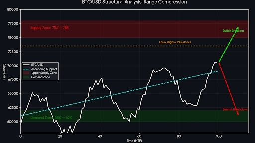
ax.plot(days, price, color='white', linewidth=2, label='BTC/USD')
# Plot steigende Trendlinie
ax.plot(x_trend, y_trend, color='cyan', linestyle='--', linewidth=2, label='Aufsteigende Unterstützung')
# Angebotszone (75K - 78K)
ax.axhspan(75000, 78000, color='red', alpha=0.2, label='Obere Angebotszone')
ax.text(5, 76500, 'Angebotszone: $75K - $78K', color='red', fontweight='bold', fontsize=12)
# Nachfragezone (60K - 62K)
ax.axhspan(60000, 62000, color='green', alpha=0.2, label='Nachfragezone')
ax.text(5, 60500, 'Nachfragezone: $60K - $62K', color='green', fontweight='bold', fontsize=12)
# Widerstandsniveau (Gleiche Hochs)
ax.axhline(73500, color='orange', linestyle=':', linewidth=2, alpha=0.7)
ax.text(70, 74000, 'Gleiche Hochs / Widerstand', color='orange', fontsize=10)
# Formatierung
ax.set_facecolor('#0e1117')
fig.patch.set_facecolor('#0e1117')
ax.spines['bottom'].set_color('white')
ax.spines['top'].set_color('white')
ax.spines['left'].set_color('white')
ax.spines['right'].set_color('white')
ax.tick_params(axis='x', colors='white')
ax.tick_params(axis='y', colors='white')
ax.set_title('BTC/USD Strukturanalyse: Bereichskompression', color='white', fontsize=16, pad=20)
ax.set_xlabel('Zeit (HTF)', color='white')
ax.set_ylabel('Preis (USD)', color='white')
# Projektionen
# Bullischer Pfad
ax.annotate('', xy=(110, 77000), xytext=(100, price[-1]),
arrowprops=dict(arrowstyle='->', color='lime', lw=3, ls='--'))
ax.text(102, 76000, 'Bullischer Durchbruch', color='lime', fontweight='bold')
# Bärischer Pfad
ax.annotate('', xy=(110, 61000), xytext=(100, price[-1]),
arrowprops=dict(arrowstyle='->', color='red', lw=3, ls='--'))
ax.text(102, 62000, 'Bärischer Durchbruch', color='red', fontweight='bold')
ax.set_xlim(0, 115)
ax.set_ylim(58000, 80000)
ax.grid(color='gray', linestyle='--', linewidth=0.5, alpha=0.3)
ax.legend(facecolor='#1e2127', edgecolor='white', labelcolor='white')
plt.tight_layout()
plt.savefig('btc_analysis_chart.png')