

« Doms? Where we’re going, we don’t need doms. »
In traditional markets, we have a Depth of Market (DOM) to see the depth of the order book: where the big buyers are, where the sellers are hiding, how far an order will push the price.
But in the Alpha market… there is no DOM. 🥶
How to place orders in geometric progression, manage risk, feel if the market is deep or shallow when we can't see the order book? 🤔
We will reconstruct an implicit depth from the price movement between the Bollinger bands, with a small discrete energy (graph / Laplacian). 💪
1. Why DOM is so valuable (and what we lose without it)
On a classic Spot pair (BTCUSDT, ETHUSDT…), the DOM gives you:
the best bids and asks,
the volumes at each price level,
the cumulative depth up to ±0.1%, ±0.5%, ±1%, etc.
For a trader, it serves to:
identify the walls (large limit order blocks),
spread a ladder of orders (geometric progression of sizes/prices),
know if a large order will move the price by 0.05% or 2%.
On the Alpha market, all this is invisible.😱
You only see the traces of transactions in the price.🤷♂️
The idea: use these traces to guess the hidden depth.💪
2. Place the price in a Bollinger tunnel
We start from a series of prices, at regular time intervals (for example every second or every minute).
2.1. Moving average and standard deviation
On a window of length (for example 20 or 60 points), we define:
Formula (1): moving average
m_L(i) = (1 / N_L) × sum for k from 0 to N_L − 1 of P_{i − k}
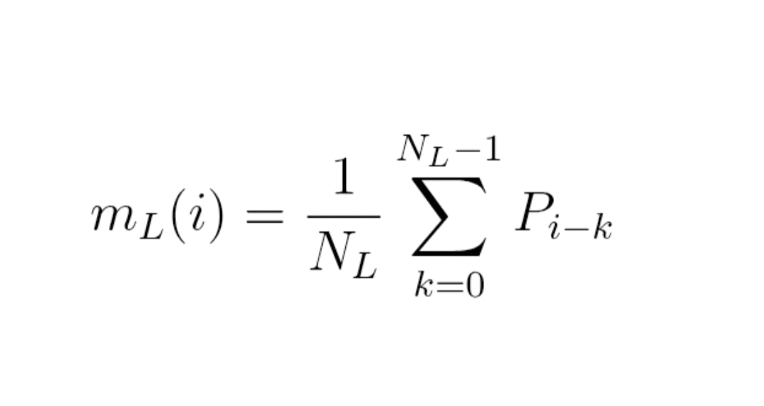
In other words,
m_L(i) = (P_i + P_{i−1} + … + P_{i−N_L+1}) / N_L.
Formula (2): moving standard deviation
σ_L(i) = square root of
[ 1 / (N_L − 1) × sum for k from 0 to N_L − 1 of (P_{i−k} − m_L(i))² ]
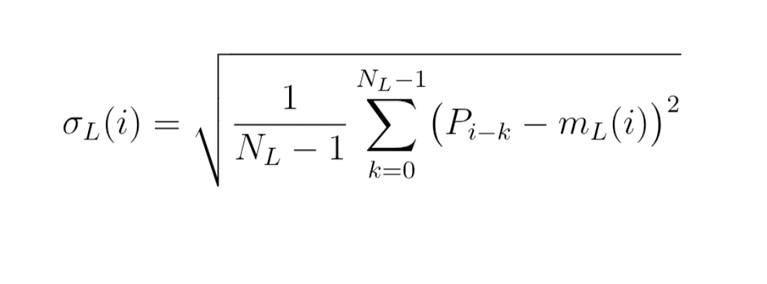
It's just the classical standard deviation, calculated on the sliding window of the last prices.
2.2. Bollinger Bands
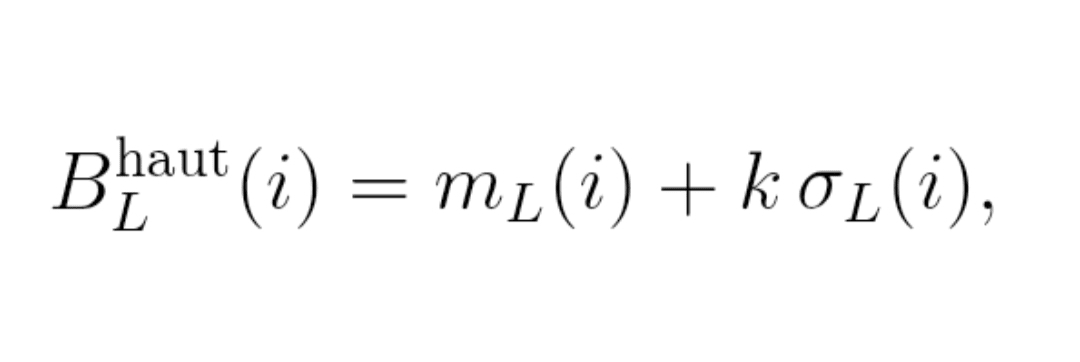
Bollinger bands at standard deviations (typically k = 2) are:
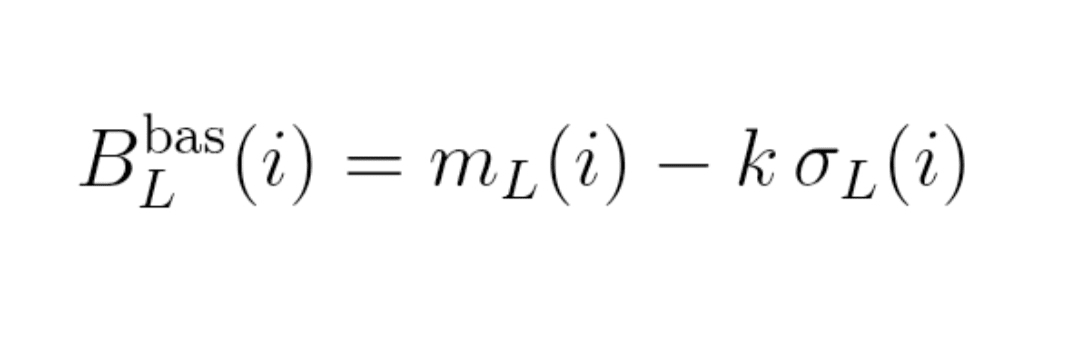
Formula (3): bands
Upper band: B_L^high(i) = m_L(i) + k × σ_L(i)
Lower band: B_L^low(i) = m_L(i) − k × σ_L(i)
2.3. Normalized price in the tunnel
We then look at where the price is in terms of number of sigmas:
Formula (4): normalized price
z_L(i) = (P_i − m_L(i)) / σ_L(i)
z_L(i) ≈ 0: price at the center of the tunnel,
|z_L(i)| ≈ 1, 2, 3: price approaching or hitting the bands.
Everything that follows happens in this normalized framework z_L.
3. Measure the 'ruggedness' of the price between the bands
Intuition:
Deep market → the price slides rather smoothly in its tunnel.
Hollow market → the price is nervous, choppy, jumps very quickly from one side to the other of the tunnel.
We measure this ruggedness with discrete Dirichlet energy.
We consider a window of indices from i_0 to i_1.
Formula (5): energy E_L
E_L(i_0, i_1)
= 1/2 × sum for i from i_0 to i_1 − 1 of [ z_L(i+1) − z_L(i) ]²
Then we normalize by the length of the window to obtain a density:
Formula (6): energy density ε_L
ε_L(i_0, i_1) = E_L(i_0, i_1) / (i_1 − i_0)
Reading:
small ε_L → rather smooth z_L trajectory,
large ε_L → very choppy z_L trajectory.
In short, ε_L measures how much the price 'wiggles' inside its Bollinger tunnel, regardless of the price scale (thanks to normalization by σ_L).
4. Implicit depth: a simple score Λ_L
We now want to link this ruggedness to market depth.
4.1. Small stylized model
We note:
Formula (7): elementary return
r_i = log(P_{i+1}) − log(P_i)
We assume a very simple model:
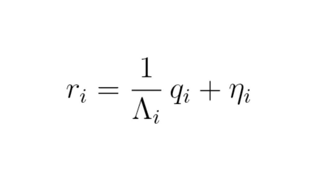
Formula (8): microstructural model
r_i = (1 / Λ_i) × q_i + η_i
where:
q_i = order imbalance (market buys − market sells) over the interval,
Λ_i = local market depth,
η_i = 'noise' (news, fundamental flow…).
Without DOM, we see neither q_i nor Λ_i.
But we see r_i, therefore z_L, hence ε_L.
By reasoning on variances and grouping constants, we arrive at a relationship of the type:
Formula (9): variance of returns (diagram)
E[r_i²] ≈ σ_q² / Λ² + σ_η²
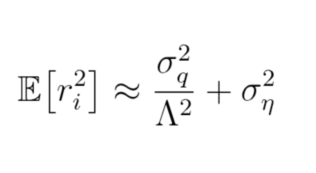
(on average over the window, σ_q and σ_η are constants, Λ the typical depth).
The key idea: the smaller Λ is, the larger the term σ_q² / Λ² is, thus the larger r_i² is → the more the price is shaken for the same order flow.
By linking z_L and r_i (z_L is roughly the return divided by σ_L), we find that ε_L increases when Λ decreases.
Thus, a very simple implicit depth score 👇
4.2. Practical definition of score Λ_L
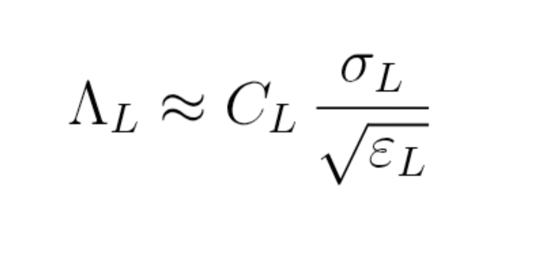
Formula (10): implicit depth score
Λ_L ≈ C_L × σ_L / square root of ε_L
where:
σ_L = local volatility,
ε_L = energy density,
C_L = constant to calibrate on a pair where the DOM is visible.
Reading:
large Λ_L → the market absorbs order flows well → strong depth.
small Λ_L → the price 'jumps' a lot for the same σ_L → hollow market.
You now have an implicit depth index without seeing the book. 🤩
5. Implied volume up to the bands
In many microstructure models, the volume needed to move the price by a certain Δp is proportional to Λ_L × |Δp|.
If we look at what happens up to the bands at k standard deviations:
Δp = k × σ_L.
We can then define an implied volume up to the bands:
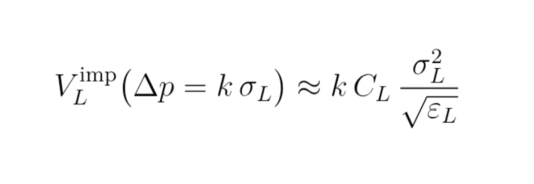
Formula (11): implied volume V_L^imp
V_L^imp (Δp = k σ_L)
≈ k × C_L × σ_L² / square root of ε_L

This V_L^imp is an order of magnitude of the volume that would be needed (on average) to sweep the hidden book up to the Bollinger bands.
On a pair with DOM, you can compare:
V_L^imp ↔ actual cumulative volume in the book.
On the Alpha market, you only have V_L^imp… but it's already a compass. 🧭
6. How to implement this on Binance
6.1. Phase 1: calibration on a pair with visible DOM
1. Choose a very liquid pair (BTCUSDT, ETHUSDT Spot).
2. In live:
retrieves prices (trades or 1s candles),
retrieves DOM snapshots (cumulative depth up to ±0.1%, ±0.5%, ±1%, etc.).
3. For each window:
calculate m_L, σ_L, ε_L,
calculate the raw indicator S_L = σ_L² / square root of ε_L,
measures the actual cumulative volume V_obs in the DOM up to Δp = k σ_L.
4. Perform a simple regression:
Formula (12): empirical relationship
V_obs ≈ C_L × S_L
(with S_L = σ_L² / √ε_L)
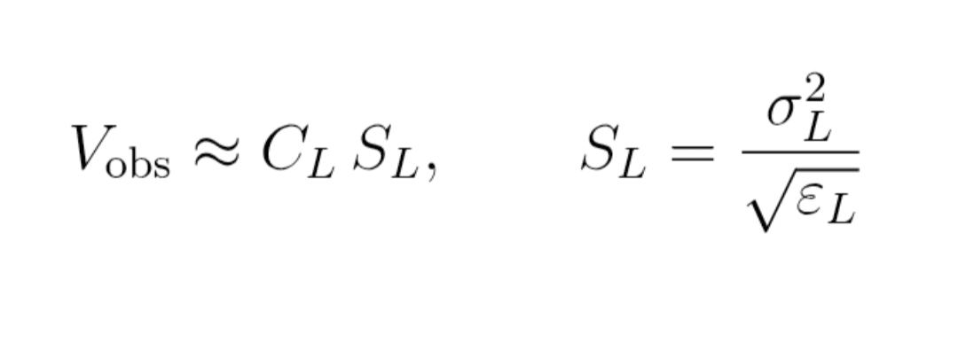
You deduce the constant C_L for this scale L.
6.2. Phase 2: application on the Alpha market (without DOM)
1. On your Alpha pair:
retrieves prices live,
calculate m_L, σ_L, ε_L.
2. Apply the formula:
Formula (13): final implied volume
V_L^imp (Δp = k σ_L) ≈ k × C_L × σ_L² / √ε_L
3. Display in real time:
the score Λ_L,
the curve Δp ↦ V_L^imp (your phantom DOM).
7. Concrete use for your orders
7.1. Build a ladder depending on Λ_L
If Λ_L is high: deep market,
you can:
bring the levels of your geometric progression closer,
keep order sizes fairly regular.
If Λ_L is low: hollow market,
you can:
space the levels further apart,
reduce the size of orders close to the price,
keep volume for further levels.
7.2. Read the implicit 'liquidity holes'
By looking at Λ_L in real time:
Λ_L drops sharply while σ_L does not change much:
alert: the market is becoming fragile,
you can reduce leverage, widen stops, avoid aggressive 'market'.
Λ_L rises after a shock:
sign of resilience: depth returns, the market recovers.
8. Limits and common sense
It is not an oracle:
does not see the spoofers,
does not include macro news,
does not replace your money management.
The indicator depends:
the choice of the window N_L,
on the quality of calibration C_L,
the granularity of the data.
To use as:
an implicit depth radar, complementing your technical analysis,
not as a magic 'buy/sell' button.
9. To go further
This article gives the 'trader' version.
Behind, there is a small theory:
function z_L viewed as a function on a chain (graph),
Dirichlet energy,
link with the heat equation and progressive smoothing.
In a separate math article, we will detail all this properly, with demonstrations supporting it on the TikTok account @Maths4Traders 💪🤩